Introduction

Consider the following problem:

$$\begin{equation} \begin{aligned} P:= \min_{x_1,x_2} & f(x_1,x_2) \\\text{s.t. } x_1x_2 &\leq 1,\\ -10x_1-x_2 &\leq -6,\\ x_1 &\in [0,1.5],\\ x_2 &\in [1,4]. \end{aligned} \end{equation}$$

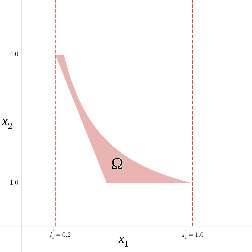
The feasible region for this problem corresponds to the red area in Figure 1, denoted as $\Omega$.

Notice that although the range of the variable $x_1$ is originally $[0,1.5]$, the feasible region in the figure only admits values of $x_1$ between $0.2$ and $1$ (red dashed lines in Figure 1). Knowing this, it is then logical to change the bounds of $x$ in the original problem from $x_1 \in [0,1.5]$ to $x_1 \in [0.2,1]$ (i.e., tightening the bounds of $x_1$).

This change will make other calculations and techniques used by Octeract Engine more effective (e.g., relaxations and branching).

In general, for a problem $\min_{x \in \Omega} f(x)$ we would like to find the tightest bounds for each variable $x_i$, i.e., find the lower bound $l_i^\star = \min_{x \in \Omega} x_i$, and upper bound $u_i^\star = \max_{x \in \Omega} x_i$.

However, unlike our previous example, it is not easy to solve the problems $\min_{x \in \Omega} x_i$ and $\max_{x \in \Omega} x_i$, and a different approach is required. Feasibility based bounds tightening (FBBT) , Optimisation based bounds tightening (OBBT) and Constraint propagation (CP), are some of the algorithmic techniques implemented in Octeract Engine to approach this important task.